Equilibrium Propagation in the Complex Domain
The main body of this work is a generalization of the proof found in Axel Laborieux's Holomorphic Equilibrium Propagation to the classic Equilibrium Propagation algorithm to derive an exact gradient estimator/nudging protocol. Demo code itself is adapted from Alex Gower's instructive OIM-Equilibrium-Propagation fork of Laborieux's OG Equilibrium-Propagation repo.
On Complex Analysis
A first course in complex analysis is typically taught as applications of holomorphic function theory. To the uninitiated, holomorphic functions are simply functions where naively "taking the derivative" makes sense in complex numbers: \[\dfrac{df}{dz}\bigg|_{z=z_0}=\lim_{\varepsilon\to 0}\dfrac{f(z_0+\varepsilon)-f(z_0)}{\varepsilon}\] Counter-intuitively, this quantity isn't actually well-defined for arbitrary complex functions who have partial derivatives in the real and imaginary components. Instead this requires a special category of differentiability just for complex numbers called holomorphy. A function \(f(x+iy)=u(x,y)+iv(x,y)\) where \(f:\mathbb{C}\to\mathbb{C}\) and \(u:\mathbb{R}\to\mathbb{R}\) and \(v:\mathbb{R}\to\mathbb{R}\) is holomorphic when \(u\) and \(v\) satisfy the Cauchy-Riemann equations: \[\dfrac{\partial u}{\partial x}=\dfrac{\partial v}{\partial y}\] \[\dfrac{\partial v}{\partial x}=-\dfrac{\partial u}{\partial y}\] Generally one should think of \(\mathbb{C}\to\mathbb{C}\) functions as \(\mathbb{R}^2\to\mathbb{R}^2\) functions, and then apply holomorphic function theory to any \(\mathbb{R}^2\to\mathbb{R}^2\) whenever the Cauchy-Riemann equations are satisfied.
Holomorphic function theory possesses an unusual amount of structure which allows for the application of powerful theorems when holomorphy can be identified in a system, such as the Cauchy differentiation formula below: \[\dfrac{d^nf}{dz^n}\Bigg|_{z=z_0}=\dfrac{n!}{2\pi i}\oint_\gamma \dfrac{f(z)}{(z-z_0)^{n+1}}dz\] Which is true when \(\gamma\) is the boundary of an arbitrary simply-connected, compact domain containing \(z_0\) where \(f\) is holomorphic.
To generalize beyond holomorphic function theory we have to weaken our requirement that the above limit is uniform regardless of the orientation of \(\varepsilon\) - this requires the introduction of the Wirtinger derivatives which can be written in terms of partial derivatives of the embedded \(\mathbb{R}^2\) system in \(\mathbb{C}\):
\[\dfrac{\partial f}{\partial z}=\dfrac12\left(\dfrac{\partial f}{\partial x}-i\dfrac{\partial f}{\partial y}\right)\qquad \dfrac{\partial f}{\partial \bar{z}}=\dfrac{1}{2}\left(\dfrac{\partial f}{\partial x} + i \dfrac{\partial f}{\partial y}\right)\]With the Wirtinger partial differential operators, we have it that we can rewrite the Cauchy-Riemann equations in the form:
\[\dfrac{\partial f}{\partial z} = \dfrac{df}{dz}\qquad \dfrac{\partial f}{\partial \bar{z}} = 0\]Symmetrically with this new definition, we can also define a notion of "anti-holomorphy":
\[\dfrac{\partial f}{\partial z} = 0 \qquad \dfrac{\partial \bar f}{\partial \bar z} = \dfrac{d \bar f}{dz}\]We can interpret the Wirtinger derivatives as a sort of decomposition of the tangents of an \(\mathbb{R}^2\) function into conformal (uniform scaling and rotation) and non-conformal parts (shear transformations).
Equilibrium Propagation
Equilibrium Propagation (EP) is an algorithm for training Energy-Based Models (EBMs) which are of great importance to the neural hardware community as they capture realistic constraints of learning with physical devices. It works by assuming that you have a model with a free energy function \(E:\mathbb{R}^n\to\mathbb{R}\) and a loss function \(\mathcal{L}:\mathbb{R}^n\to\mathbb{R}\) with a nudging factor \(\beta\in\mathbb{R}\) which are combined linearly to give the total EP energy F such that the dynamics of the system are given by:
\[\dfrac{dz_i}{dt}=-\dfrac{\partial F}{\partial z_i}\]In general training proceeds by running these dynamics to an infinite-time equilibrium in both a "free" phase \((\beta=0)\) and a "nudged" or "clamped" phase \((\beta > 0)\). The remarkable result of Equilibrium Propagation is that the local states of neurons at these two equilibria at the limit \(\beta\to 0\) encode the exact gradient that we would expect to see in backpropagation through time at equilibrium.
\[\dfrac{\partial\mathcal{L}}{\partial\Theta}\approx \dfrac{1}{\beta_0}\left(\dfrac{\partial F}{\partial\Theta}\bigg|_{\beta=\beta_0}-\dfrac{\partial F}{\partial\Theta}\bigg|_{\beta = 0}\right)+O(\beta_0)\]Note: Intuitively, this is the limit definition of the \(\beta\)-partial derivative of \(\partial F/\partial \Theta \). And since \(F\) is typically defined by a local product of neural states and their weights and biases - we get local estimators of gradients.
However this exactness comes with a physical cost, namely that using a small \(\beta\) requires high-precision control. This requires prohibitively expensive nudging devices which are at a premium in silicon. Thus using equilibrium propagation splits researchers into one of three camps:
- Take the hardware penalty and use the algorithm as is
- Find out just what you can get away with in cheaper hardware
- Explore variations of equilibrium propagation with higher precision with large nudging factors
This work falls into camp 3, and to explain where we are and where we're going I'll have to relate the work of Axel Laborieux:
The Work of Axel Laborieux
Two papers of Axel's standout as contributions to answering the question: "how might we use a bigger \(\beta\) in eqprop while retaining precision". The first of these works is the symmetric nudging protocol, which improves the error substantially by leaning into the theory finite difference methods of numerical differentiation:
\[\dfrac{\partial \mathcal{L}}{\partial \Theta}\approx\dfrac{1}{2\beta_0}\left(\dfrac{\partial F}{\partial \Theta}\bigg|_{\beta=\beta_0}-\dfrac{\partial F}{\partial \Theta}\bigg|_{\beta=-\beta_0}\right)+O(\beta_0^{2})\]One should note that similar formulas exist to arbitrary precision where the \(c_k\) can be computed with Taylor expansion matching:
\[\dfrac{\partial \mathcal{L}}{\partial \Theta}\approx \dfrac{1}{\beta_0}\sum_{k=1}^N c_k \left(\dfrac{\partial F}{\partial \Theta}\bigg|_{\beta= k\beta_0}-\dfrac{\partial F}{\partial \Theta}\bigg|_{\beta= -k\beta_0}\right)+O(\beta_0^{2N})\]And the second is holomorphic equilibrium propagation which provides arbitrary precision in the complex plane with the use of the Cauchy differentiation formula where \(\gamma\) is some contour in \(\beta\) bordering a subset containing \(\beta=0\):
\[\dfrac{\partial \mathcal{L}}{\partial \Theta}=\dfrac{1}{2\pi i}\oint_\gamma \dfrac{\partial F}{\partial \Theta}\dfrac{d\beta}{\beta^2}\]As well as an estimator of this contour integral using a circular path of radius \(|\beta_0|\) centered at \(\beta=0\) with \(N\) points \(\beta_k=|\beta_0|\exp(2\pi i k/N)\):
\[\dfrac{\partial \mathcal{L}}{\partial \Theta} \approx \dfrac{1}{2\pi |\beta_0|^2N}\sum_{k=1}^N\dfrac{\partial F}{\partial \Theta}\bigg|_{\beta=\beta_k}\beta_k + O(|\beta_0|^N)\]The machinery of holomorphic equilibrium propagation requires that \(F\) itself is holomorphic or in other words that dynamics are conformal. So despite the fact HEP works with arbitrary large contour integrals, this imposes a large constraint on the applicability of HEP to complex dynamics and raises an interesting question of how one might generalize it.
Holomorphic Equilibrium Propagation on Locally Conformal Dynamics
To generalize Holomorphic Equilibrium Propagation formula, it's important to remember that the equilibrium points \(z^*\) of our dynamics are a function of \(\beta\) and therefore so to are \(E\) and \(\mathcal{L}\). This is the basis of the holomorphic implicit function theorem and it explains how the holomorphic equilibrium propagation formula arises from supposedly disconnected nudging and energy.
Namely, at equilibrium \(z^*\) of determined by holomorphic \(F\) we have that \(\partial_z F = 0\) (shorthand for partial derivative in z), then if \(\partial_{\Theta,\beta}\partial_z F\) defines an invertible matrix - it follows there is a holomorphic "implicit function" \(g\) such that \(g(\Theta,\beta)=z^*\) satisfying \(\partial_z F = 0\)
In order that we may apply Cauchy's integral formula, it holds that \(g\) must not just be once-differentiable but satisfy the Cauchy-Riemann equations. Thus the only valid generalization possible is to locally holomorphic \(g\) induced by a locally holomorphic \(F\). In this case, there exists a small neighborhood around \(\beta=0\) such that \(\bar\partial_z F < \varepsilon\) in which we can use all of the HEP tools as intended plus this error term.
Unfortunately, we lose the large finite \(|\beta|\) for arbitrary precision, but we do recover a notion in which these tools can be used in locally holomorphic energy functions. Fortunately, so long as we can prove this local holomorphy - we can keep the HEP algorithm.
Specifically in the case of loss, I'm assuming that \(\mathcal{L}(y,\hat y)= \sum|y-\hat y|\) and so we have nudging dynamics -\(\partial \mathcal{L}/\partial \bar{y} = \hat y - y\). We note a couple things, first of all the dynamics flow to minimize anti-holomorphic contributions and at equilibrium, ie. \(\beta\bar\partial_z \mathcal{L}=\bar\partial_z E\) that it also holds that \(\beta\partial_z \mathcal{L}=\partial_z E\) if \(E\) is real-valued, since \(\mathcal{L}\) is real-valued too.
The Stuart-Landau Coupled STNO Model
Spin-Torque Nano-Oscillators (STNOs) can be simulated using coupled Stuart-Landau dynamics, we assume the \(|z|=\)amplitude and \(\arg(z)\)=phase representation and assume that all oscillators have the same frequency, and that we are observing them in a rotating frame where coupling coefficients \(J_{ab},h_a\in\mathbb{R}\):
\[\dfrac{dz_a}{dt} = (1-z_a\bar{z}_a)z_a+\sum_{a\neq b} J_{ab}(z_b-z_a)+h_az_a\]To intuit how complex dynamics generally work, the real component times variable corresponds to radial velocity and imaginary component time the variable is rotational velocity around the complex origin, so we can rewrite these equations into their polar form given by:
\[\frac{dr_a}{dt} = (1 - r_a^2)r_a + \sum_{b\neq a} J_{ab}[r_b \cos(\theta_b - \theta_a) - r_a] + h_ar_a\] \[\frac{d\theta_a}{dt} =\frac{1}{r_a}\sum_{b\neq a} J_{ab} r_b \sin(\theta_b - \theta_a)\]We note that this is reminiscent of Kuramoto oscillators and that our choice of biasing implies amplitude biasing rather than conventional phase biasing. To bend these into an EBM, we require an energy \(F:\mathbb{C}^n\to\mathbb{R}\) such that \(dz/dt=-\partial F/\partial \bar z\) and \(z\to z^*\) as \(t\to \infty\) - the choice of the conjugate Wirtinger derivative means that dynamics move to minimize non-holomorphic contributions. In particular since \(F\) is real-valued when we have \(\partial_z F=0\) it implies that also \(\bar\partial_z F =0\) and as you can see this simplifies stability analysis substantively, we will define the components such that \(F=E+\beta\mathcal{L}\), we note that \(|z|=\sqrt{z\bar z}\):
\[E(z;\Theta) = -\sum_a (|z_a|^2 - \tfrac{1}{2}|z_a|^4) - \tfrac{1}{2}\sum_{a\neq b}J_{ab}|z_b-z_a|^2 - \sum_a h_a |z_a|^2\] The argument \(F\) is locally holomorphic in \(\beta\) at equilibrium relies on the fact that we expect to see Kuramoto-esque phase-locking behavior as well a parallel notion of amplitude locking - infinitesimal variations in \(\beta\) simply shift the equilibrium points either radially or rotationally due to Stuart-Landau oscillator's circular limit set, these maps in their infinitesimal limit are given by a simple per-oscillator complex multiplication, each of which are seperately locally holomorphic.To complete the argument and make it appropriate for holomorphic implicit function theorem, we have it by Hartog's theorem that this seperate local holomorphy in all parameters implies the system is jointly locally holomorphic and so the holomorphic implicit function theorem can be used in this small domain.
Therefore, this model encodes a locally holomorphic energy and we may use HEP tools in the case of small \(|\beta|\). We note that this argument could be similarly extended to other non-linear oscillators, however, this approximation suffers with non-linear distortion and requires analysis.
STNO Demonstration
A simple way to demonstrate local holomorphy is to actually attempt naive equilibrium propagation on this system. The fact that this works at all, is an indication of locally conformal dynamics.
Why is that so? What we've seen from the prior argument is that a system of \(N\) oscillators is structured with \(2N\) parameters - therefore, a proper estimator would be parameterized in all of these \(2N\) parameters, however, we can get away with estimating on just \(N\) which is only possible in locally holomorphic equilibria.
Anecdotally, having spoken to other oscillator ising machine heads, equilibrium propagation is tempermental on non-linear oscillator systems. This again has a simple explanation from the complex analysis, local holomorphy is weaker in the non-linear case, so any gradient estimator must capture all \(2N\) degrees of freedom - naively assuming you can just propagate equilibrium in the voltage delta or phase alone in the non-linear case does not work well.
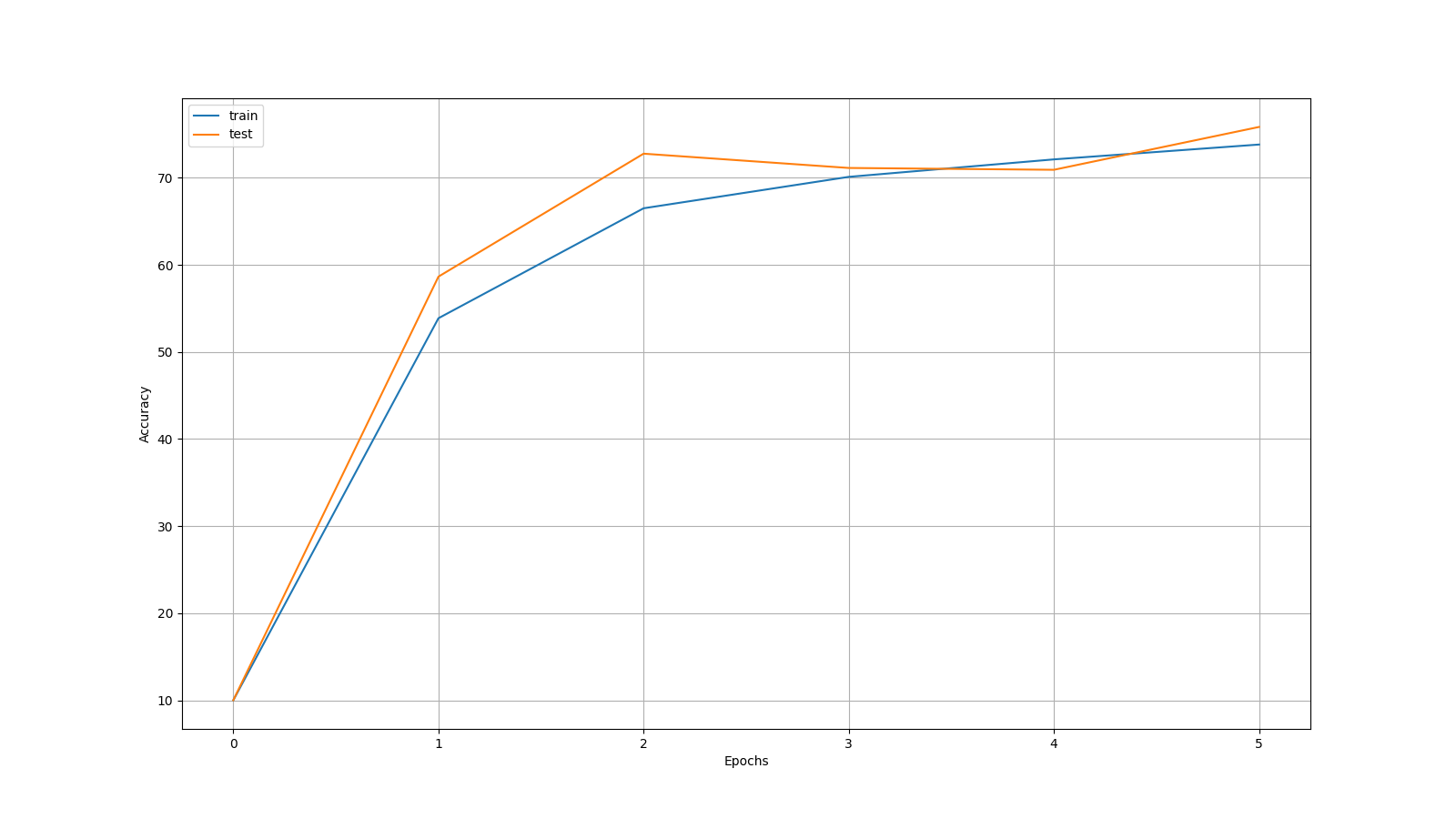
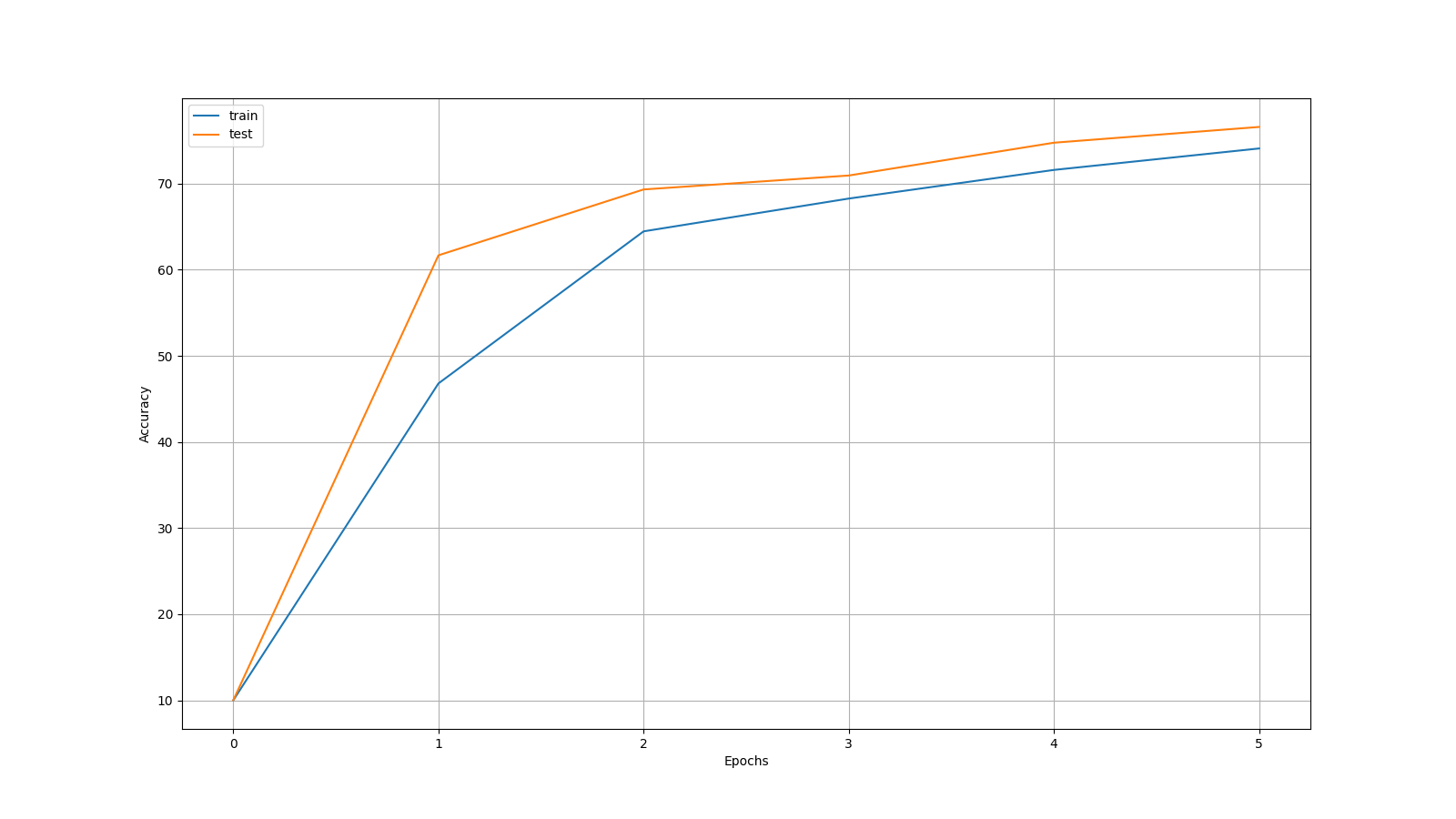
Here is a demonstrator with the STNO 784-256-10 system which you can find in my repository using amplitude coupling instead of phase coupling - we train it for 5 epochs on MNIST and FMNIST with symmetric equilibrium propagation - training is slow and unstable because of complex differentiation overhead, the implicit numerical schemes for dubious stability and sometimes the model can collapse either due the Stuart-Landau phenomenon of "amplitude death" or numerical explosion. Here's one that worked!
The Kuramoto Model in Complex Coordinates
As an academic curiosity, another possible angle is to approach it from a more mathematically pure perspective that is "ampltiude agnostic" using the Kuramoto model. It is possible to realize the Kuramoto model in terms of complex functions by using the change of coordinates between polar and Wirtinger coordinates - the result is that energy is given by:
\[\dfrac{\partial E}{\partial \theta_i}\dfrac{\partial \theta_i}{\partial \bar{z}}=\dfrac{i}{r}\sum_{ab}J_{ab}\sin(\theta_b-\theta_a)(\cos(\theta_i)-\sin(\theta))\] \[\implies E=\dfrac{i}{4}\sum_{a,b} \dfrac{J_{ab}}{|z_b|}\left(\dfrac{\bar{z}_a^2 z_b}{z_a^2\bar{z}_b}-\dfrac{\bar{z}_b}{z_a}\log(\bar{z}_a^2)\right)\]
This form unsurprisingly restricts the energy to terms of the unit circle of individual \(z_a\) and \(z_b\) and is holomorphic in the sense that there is only the unit circle perturbations to the logarithm of \(\bar{z}_a^2\) which is itself holomorphic in local neighborhoods (although, it is techically a double helix Riemann surface, so you have to pick your spiral and your height on the spiral and do your calculus roughly there).
This is not nice and real like the Stuart-Landau model is, but one can verify that \(\partial \bar{E}/\partial z = \partial E/\partial \bar{z}\) which reaffirms the equilibration property on the complex plane \(\partial_z E = 0 \iff \bar\partial_z E = 0\), that such a zero exists follows from the fact that when normal Kuramoto dynamics converge that our dynamics remain well-behaved - although what \(|z|\) represents in this picture is beyond me. This model has not been studied to the best of my knowledge.
Given that these dynamics equilibriate and that all perturbations result in linear combinations of unit vectors multiplied with log curve - this too represents a locally holomorphic function in \(\beta\).
Non-Holomorphic Equilibrium Propagation
Where local holomorphy fails, Green's theorem begins to apply - we do have an alternative means to construct arbitrary precision estimators but these unfortunately are \(O(\beta_0^{\sqrt{N}})\) if we naively estimate the surface integral with a grid.
In short this can only be handled by acknowledging the presence of the 4 point nudging estimator in the two cardinal directions governing a non-linear oscillators dynamics - the simplest choice of coordinates would probably be the polar coordinates as in most models these correspond to measurable quantities like phase and amplitude or frequency modulation.
I've attempted to tame a van der Pol oscillator system with this insight in my repository it requires RK4 for any kind of stability and needless to say, it isn't going very well, but its there if anyone feels like fighting cursed dynamics.
Although derivations with fancy Cauchy-Pompieu machinery are certainly possible, and I include them here if anyone feels like chasing the mathematical dragon:
The \(\bar\partial\) (pronounced "del-bar") operator admits a definition due to Dimitrie Pompeiu in 1912:
\[\dfrac{\partial f}{\partial \bar z}\Bigg|_{z=z_0} = \lim_{r\to 0} \dfrac{1}{2\pi r^2}\oint_{\Gamma(z_0,r)} f(z) dz\]Where \(\Gamma(z_0,r)\) is the circular path of radius \(r\) centered at \(z_0\) - it measures quite literally strength of the failure of Cauchy's theorem at \(z_0\). This definition then lead Pompeiu in 1913 to develop an extension of Cauchy integral formula in general once-Wirtinger-differentiable complex functions reminiscent of Green's theorem over a simply-connected, compact domain \(G\):
\[f(z)=\dfrac{1}{2\pi i}\oint_{\partial G} \dfrac{f(\zeta)}{\zeta - z}d\zeta - \dfrac{1}{\pi}\iint_G \dfrac{\partial f}{\partial \bar{z}} \dfrac{dx\wedge dy}{\zeta-z}\]The failure of holomorphy means that the relationship between derivatives and integrals becomes increasingly perilous as we move to higher derivatives - however, mercifully, in the first derivative we only require that the second term becomes a "Cauchy Principal Value" with the following form due to Ilya Vekua in his book in 1962 - I will allow the real complex analysts to correct my Soviet mathematical history:
\[\dfrac{\partial f}{\partial z}\bigg|_{z=z_0} = \dfrac{1}{2\pi i}\oint_{\partial G} \dfrac{f(\zeta)}{(\zeta - z_0)^2} dz -\dfrac{1}{\pi}\iint_G \dfrac{\partial f}{\partial \bar z}\dfrac{dx \wedge dy}{(\zeta-z_0)^2} \quad(\text{p.v.})\]A Cauchy Principal Value is just an analytic technique to handle singularities, where \(C\) is a domain and \(C(\varepsilon)\) is just C with hole centered on the singularity of radius \(\varepsilon\):
\[\text{p.v.}\int_C f(z)dz = \lim_{\epsilon\to 0^+} \int_{C(\epsilon)} f(z) dz \]For any numerical work we'd like to do this basically means evaluate at the boundary first and spiral inwards becoming more hesitant as we approach the singularity.